
HyClus Viz
Published:
Hyperspectral imaging produces data cubes with hundreds of spectral bands per pixel, creating a fundamental dimensionality reduction and visualization challenge: how do you compress this high-dimensional spectral information into compact representations that preserve meaningful structure for mineral identification and sample provenance discrimination? HyClusVi addresses this problem by combining deep autoencoders with nonlinear embedding techniques (t-SNE) to transform raw spectral data into interpretable low-dimensional visualizations, enabling clustering and classification of mineral samples from industrial comminution circuits.

The Context
This project originated in the first edition of the Data Science Project course (CC5214) at the Department of Computer Science, Faculty of Physical and Mathematical Sciences, Universidad de Chile. Our laboratory proposed the project “Clusterization and Identification of mineral species from Hyperspectral images”, and three students worked on the formulation, analysis, and evaluation of the system using real data: monthly composites from comminution feeders of three different productive sectors of a large mining company operating nationwide.
The students researched and implemented deep learning systems for the analysis of high-dimensional hyperspectral images. This work complemented scientific and visualization tools that we were actively promoting and disseminating in the national mining industry. The resulting techniques for visualizing clustering results at scale have since improved our results reporting system.
The data
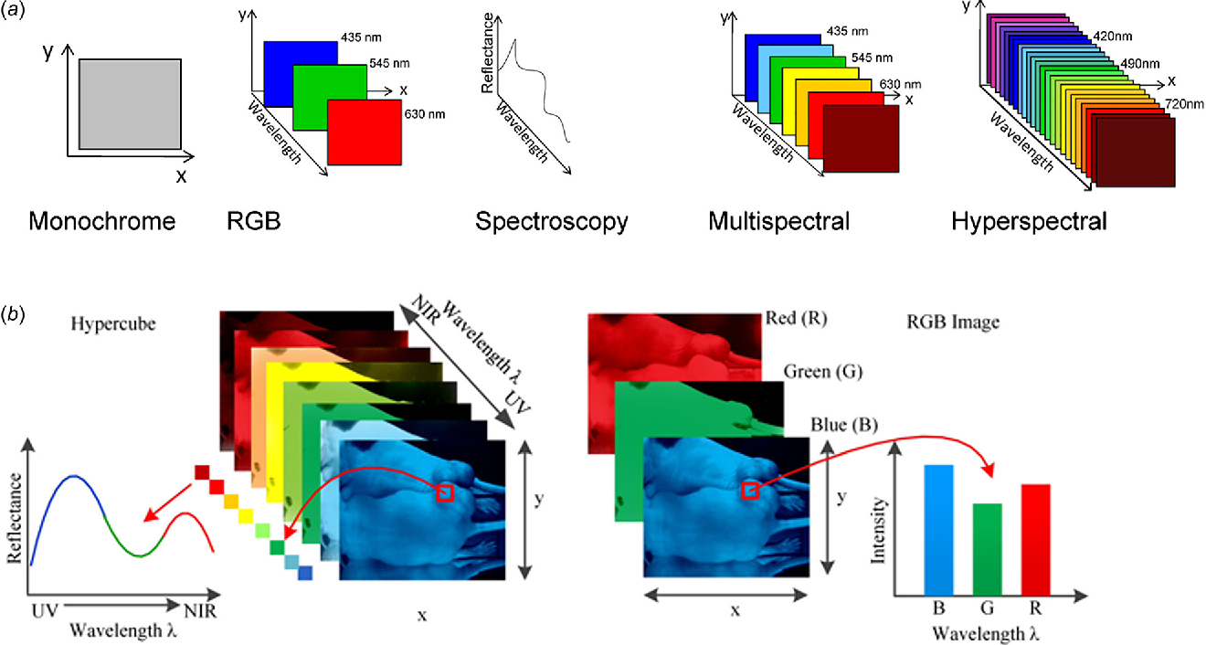
We work with hyperspectral image data. In these images, information on the spatial distribution of objects is combined with a deep characterization of the electromagnetic reflection of their components in hundreds of different bands of the spectrum.
The acquisition System
We have two hyperspectral cameras. Each one is a scanline of hundreds of spatial pixels. One camera provides information in the VNIR (between 400 and 1000 nm), while the second provides bands in the SWIR (between 1000 and 2500 nm). 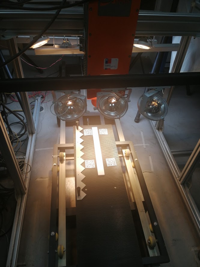
We have a mounting system for both cameras that allows them to be positioned on a conveyor belt. On this tray it is possible to position a variety of containers to handle various types of samples. 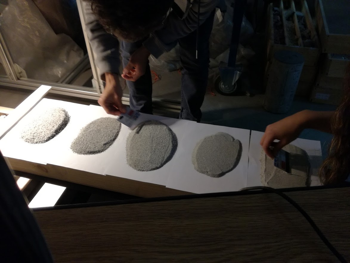
The system is complemented with a set of lighting with halogen and Led sources in order to appropriately cover the reflectance spectrum in which the cameras can acquire information. 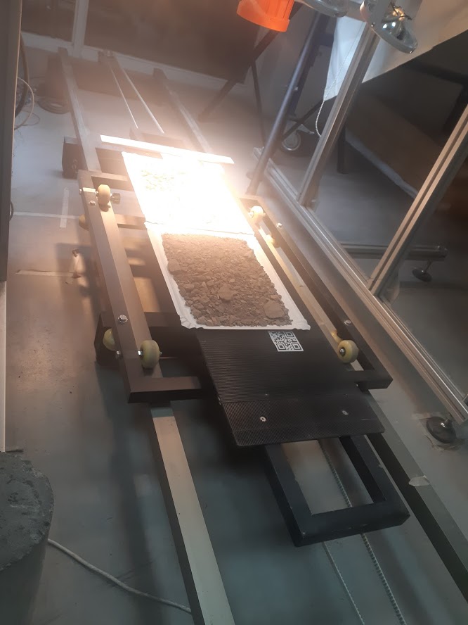
The acquisition
We have a set of samples, each characterized with DRX and DRF laboratory analysis. Due to the scope of this project, we will leave this information aside for the moment. Focusing only on the clustering of the data.
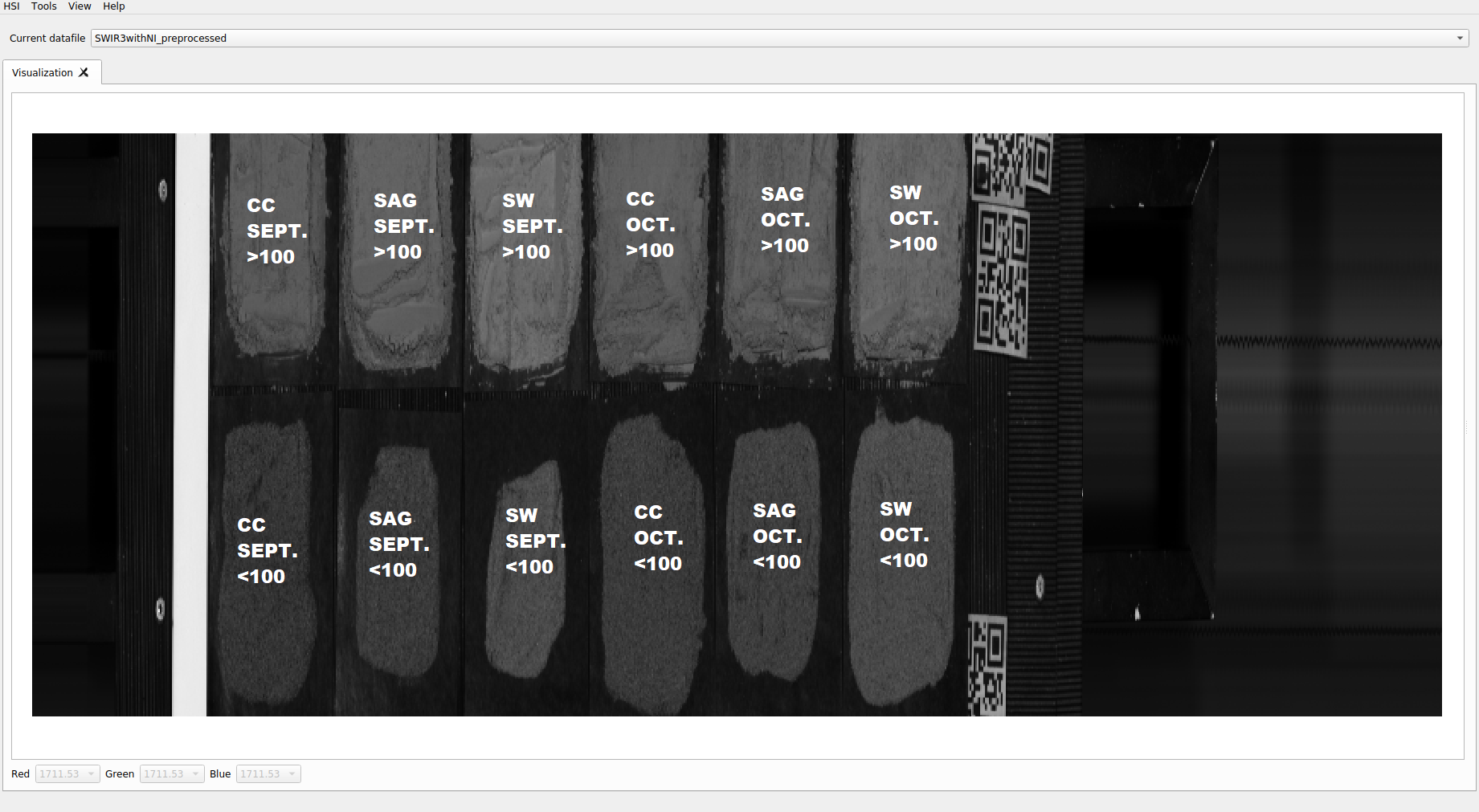
The set corresponds to one sample per month (monthly composition) during the year 2018. Furthermore, each sample comes from 3 different plants, and in two levels of different size.
This generates a set of 72 samples. Each sample is a set of granulated material.
For its hyperspectral characterization, a group of trays is distributed on the tray.
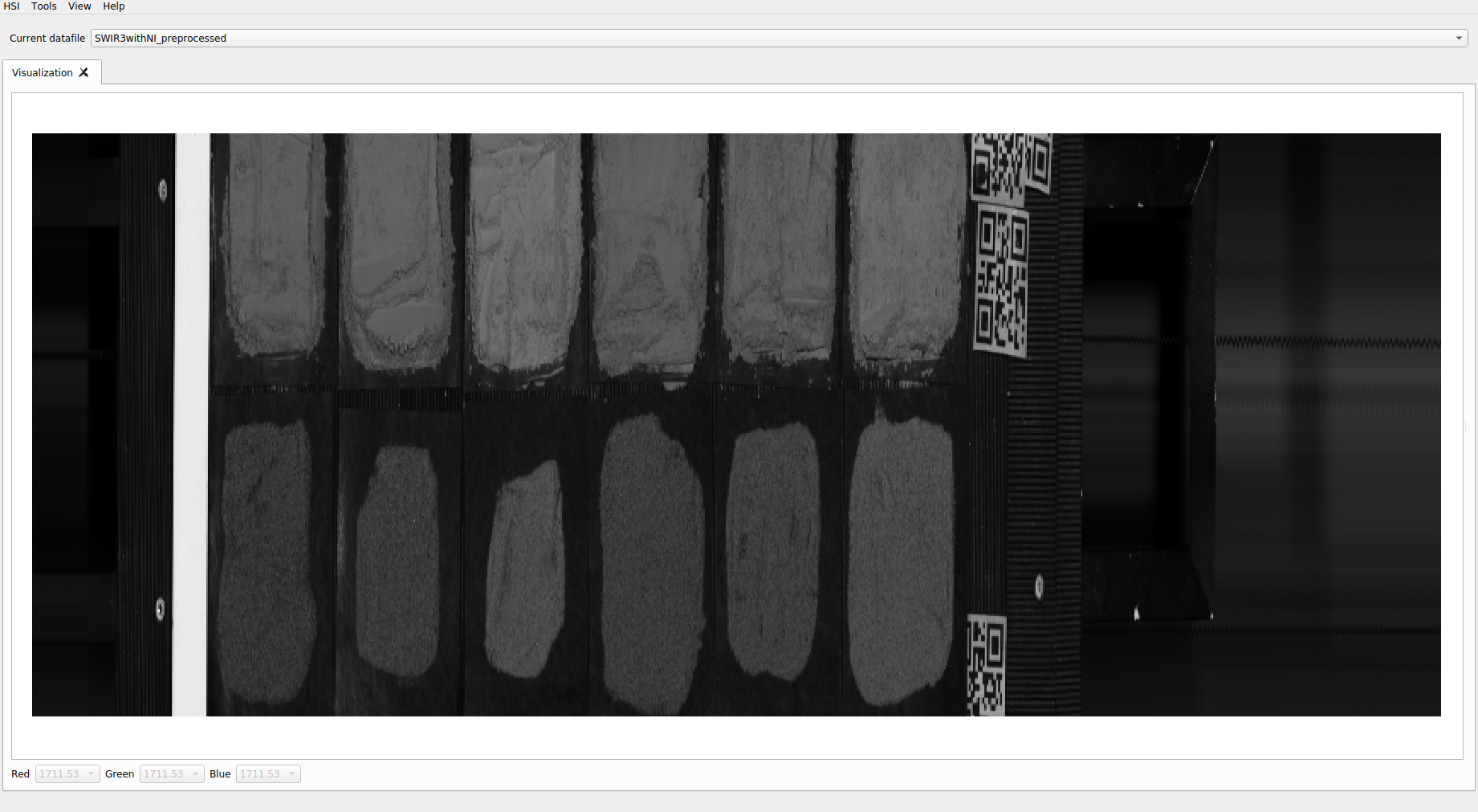
Mapping the distribution of the samples is maintained
In this way it is possible to segment and define the samples individually. From the captured image, individual containers are generated in HDF5 with each sample.
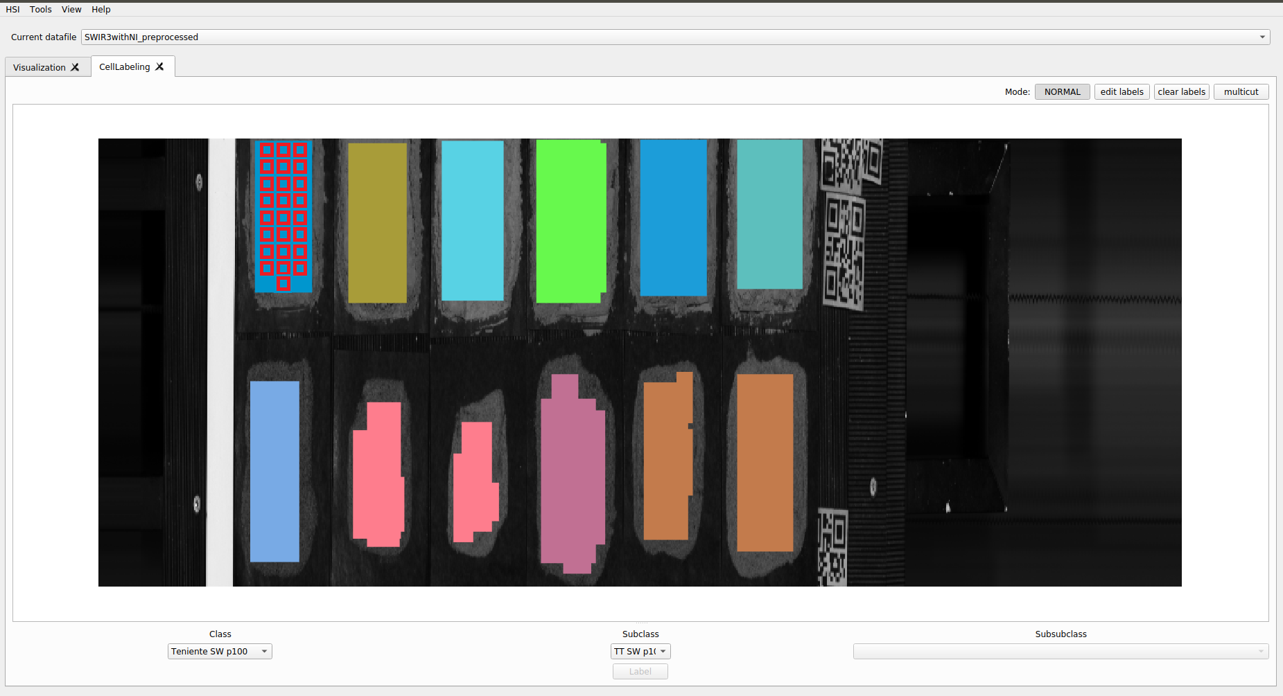
Normally these containers, for each sample, provide a hyperspectral image that preserves both spatial and spectral information.
For this analysis we will omit the spatial information, only keeping the isolated spectra for each sample. This is possible due to the level of crushing of the material, since most of the spatial correlations have been lost at this level of pulverization.
The Clustering and Visualization
Samples
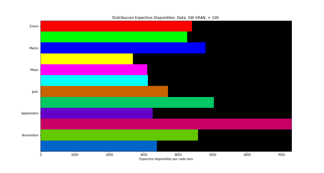
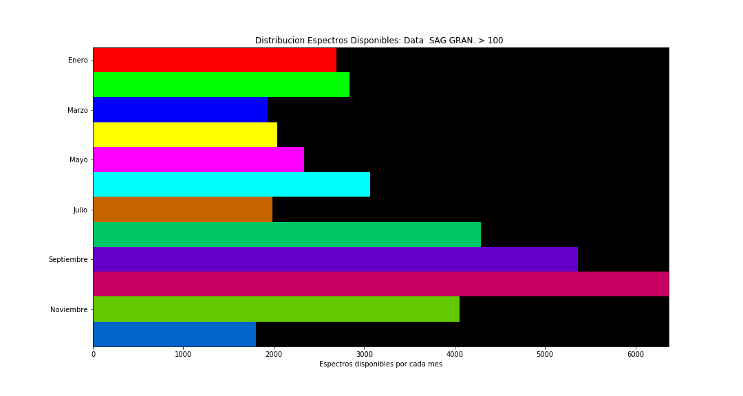
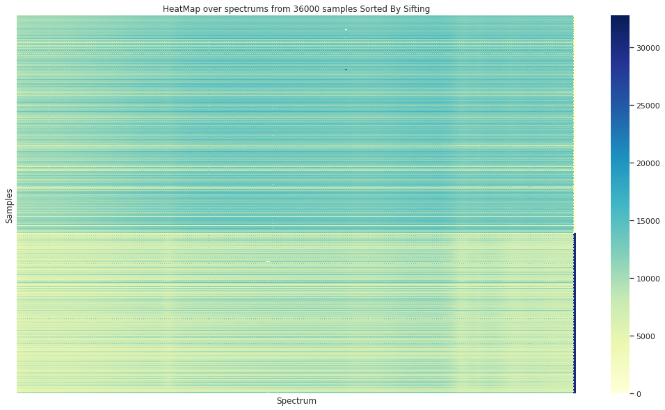
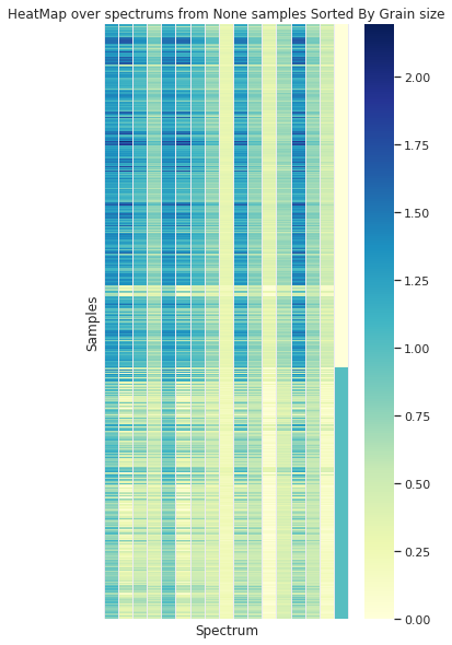
At this stage, for each granulometry level (average grain size in the sample), for each plant, and for each month, a number of pixels (spectra) are available that characterize the sample. Some of the distributions of the number of spectra are presented (more detailed information is confidential due to the origin of the data).
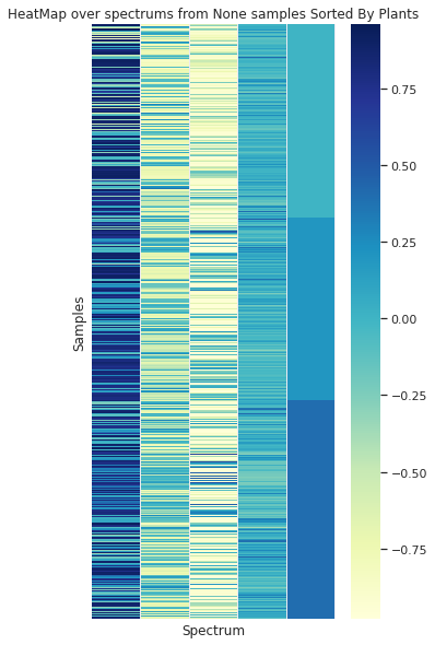
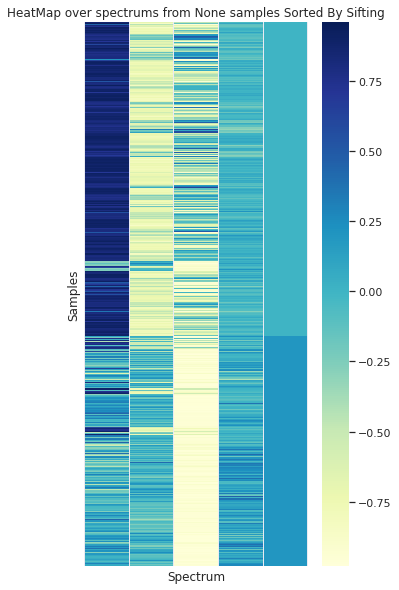
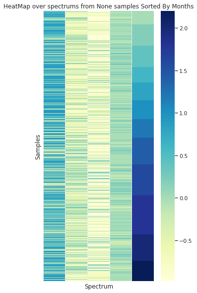
Spectra Examples
The spectral content of the samples is homogeneus, so clasical endmember identification is not a robust approach. In addition data is altered by enviromental conditions and outliers.
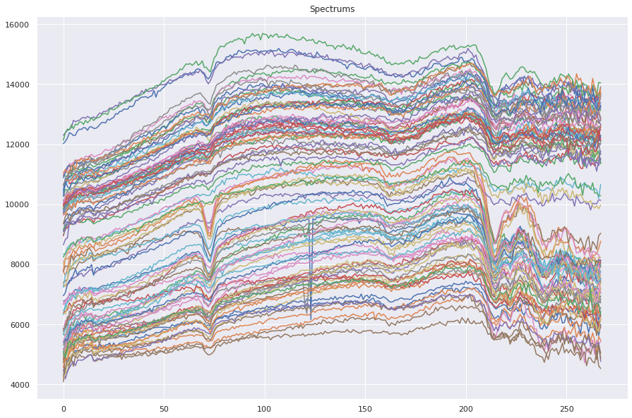
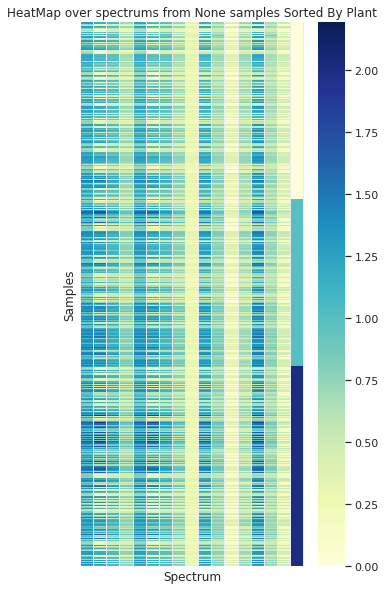
Showing some spectra organized by the 3 plants (in the vertical axis) is clear that no simple separation of the data in this domain can be achieved without processing the info
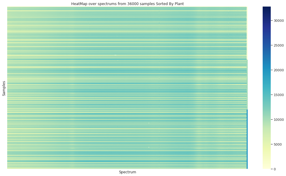
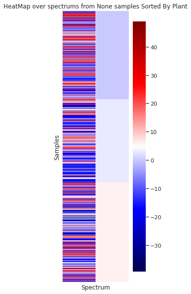
In the case of the granulometry (the grain sample size) a visual difference can be appreciated between the to groups
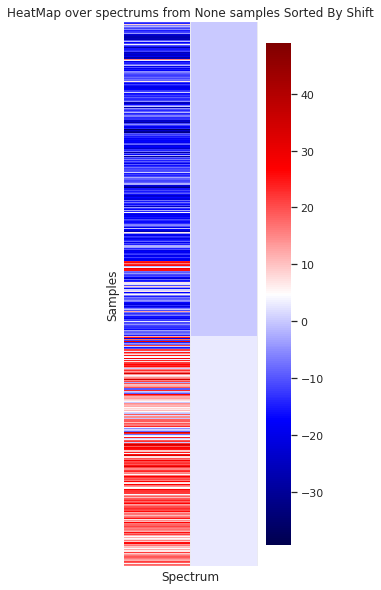
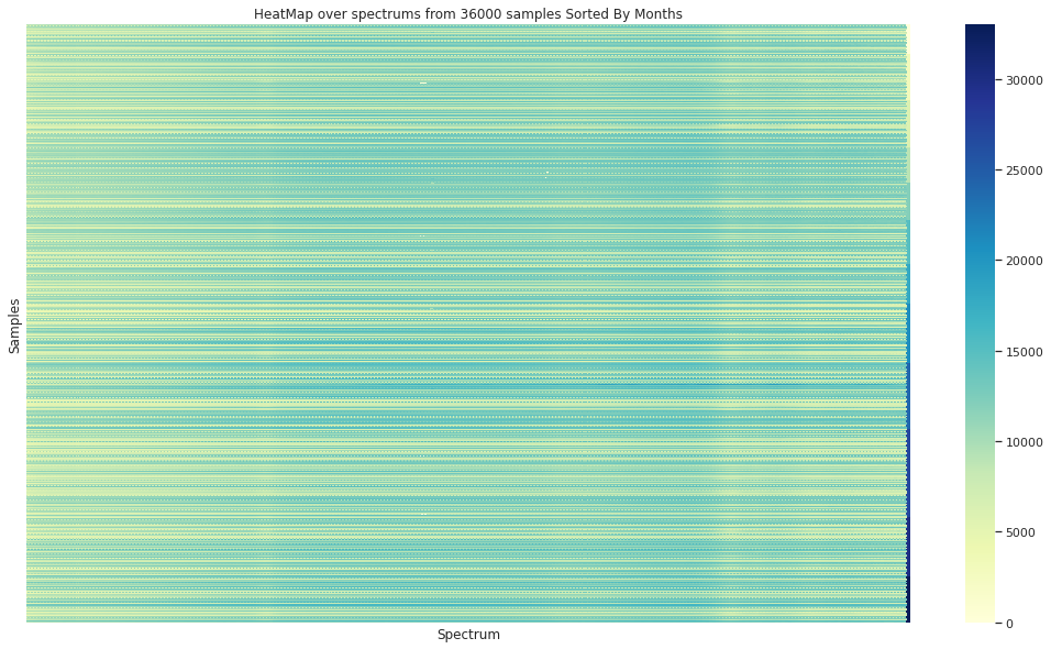
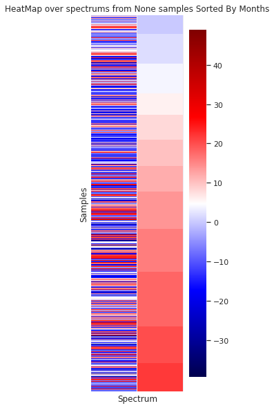
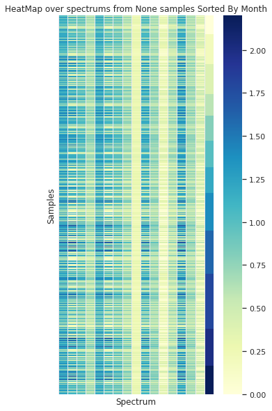
In the case of sorting the spectra by the origin month, no visual organization is observed
Deep Autoencoders
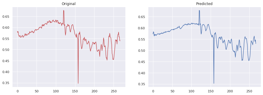
The core dimensionality reduction engine is a symmetric dense autoencoder. Each individual spectrum serves as the input, and the network learns a compressed latent representation through a bottleneck architecture. The encoder path progressively reduces dimensionality (input → 128 → 64 → 32 → 16 → 4), and the decoder mirrors this structure (4 → 16 → 32 → 64 → 128 → output). All hidden layers use tanh activation with orthogonal kernel initialization, which helps preserve gradient flow and avoid degenerate representations. Input spectra are normalized with MinMaxScaler before training, and the output layer uses sigmoid activation with binary cross-entropy loss. The bottleneck of 4 dimensions was chosen as an aggressive compression target; a second variant with 16 latent dimensions was also evaluated for comparison.
from tensorflow.keras import layers, models, callbacks
from sklearn.preprocessing import MinMaxScaler, minmax_scale
X_max_min = MinMaxScaler().fit_transform(X)

_input = layers.Input(shape=(X.shape[1],))

encoded = layers.Dense(128, activation='tanh', kernel_initializer='orthogonal')(_input)
encoded = layers.Dense(64, activation='tanh', kernel_initializer='orthogonal')(encoded)
encoded = layers.Dense(32, activation='tanh', kernel_initializer='orthogonal')(encoded)
encoded = layers.Dense(16, activation='tanh', kernel_initializer='orthogonal')(encoded)


encoded = layers.Dense(4, activation='tanh', kernel_initializer='orthogonal')(encoded)

encoded = layers.Dense(16, activation='tanh', kernel_initializer='orthogonal')(encoded)
encoded = layers.Dense(32, activation='tanh', kernel_initializer='orthogonal')(encoded)
decoded = layers.Dense(64, activation='tanh', kernel_initializer='orthogonal')(encoded)
decoded = layers.Dense(128, activation='tanh', kernel_initializer='orthogonal')(decoded)
decoded = layers.Dense(X.shape[1], activation='sigmoid')(decoded)

autoencoder = models.Model(_input, decoded)
autoencoder.compile(optimizer='rmsprop', loss='binary_crossentropy')
With the respective fitting:
kwargs = dict(monitor='val_loss')
kwargs.__setitem__('patience', 5)
kwargs.__setitem__('verbose', 1)

_early = callbacks.EarlyStopping(**kwargs)

kwargs = dict(monitor='val_loss')
kwargs.__setitem__('patience', 3)
kwargs.__setitem__('min_lr', 1e-6)
kwargs.__setitem__('verbose', 1)
kwargs.__setitem__('mode', 'auto')

learnig_rate = callbacks.ReduceLROnPlateau(**kwargs)

_callbacks = [_early, learnig_rate]

autoencoder.fit(X_max_min, X_max_min,
                epochs=30, verbose=2,
                batch_size=256, callbacks=_callbacks,
                shuffle=True,
                validation_split=0.1)
Epoch 00021: ReduceLROnPlateau reducing learning rate to 1e-06.
1101/1101 - 8s - loss: 0.6287 - val_loss: 0.6062
Epoch 22/30
1101/1101 - 8s - loss: 0.6287 - val_loss: 0.6062
Epoch 23/30
1101/1101 - 9s - loss: 0.6287 - val_loss: 0.6062
Epoch 24/30
1101/1101 - 8s - loss: 0.6287 - val_loss: 0.6062
Epoch 25/30
1101/1101 - 8s - loss: 0.6287 - val_loss: 0.6062
Epoch 26/30
1101/1101 - 8s - loss: 0.6287 - val_loss: 0.6062
Epoch 27/30
1101/1101 - 8s - loss: 0.6287 - val_loss: 0.6062
Epoch 28/30
1101/1101 - 8s - loss: 0.6287 - val_loss: 0.6062
Epoch 29/30
1101/1101 - 8s - loss: 0.6287 - val_loss: 0.6062
Epoch 30/30
1101/1101 - 8s - loss: 0.6287 - val_loss: 0.6062
<tensorflow.python.keras.callbacks.History at 0x7fbcc7ac5208>
Reduced Spectra by Autoencoder (4 bands)
After the encoded representation of the data, it is possible to recreate the visualization of the spectra grouped by the avaible categories.
Grouped by Plant
Grouped by Size
Grouped by Month
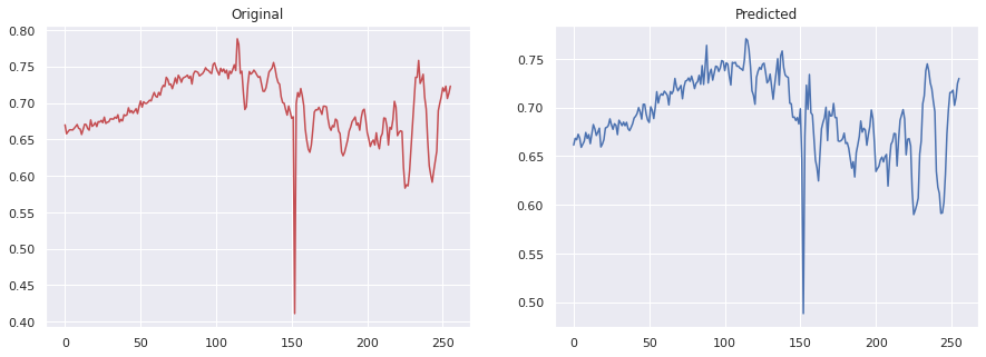
Example of a decoded spectrum from the autoencoder
Reduced Spectra by Autoencoder (16 bands)
Again, it is possible to recreate the visualization of the spectra grouped by the avaible categories for the data encoded to 16 bands.
Grouped by Size
Grouped by Plant
Grouped by Month
Example of a decoded spectrum from the autoencoder
TNSE
T-distributed Stochastic Neighbor Embedding(t-SNE) lies in the category of unsupervised dimensionality reduction techniques, that applies a non-linear dimensionality reduction approach where the focus is on keeping the very similar data points close together in lower-dimensional space.
The approach was developed as an unsupervised machine learning algorithm for visualization by Laurens van der Maaten and Geoffrey Hinton. It is relevant that outliers do not impact t-SNE.
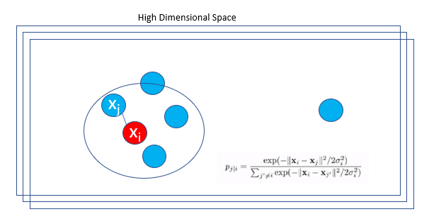
In this strategy, the probability density of a pair of points is proportional to its similarity. For nearby data points,
\[ p(j | i) \]
will be relatively high, while for points widely separated, p(j | i) will be lower.
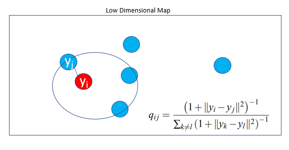
A central stage of the technique requires to find a low-dimensional data representation that minimizes the mismatch between Pᵢⱼ and qᵢⱼ using gradient descent based on Kullback-Leibler divergence(KL Divergence)
More details can be found in the repository of the t-SNE project, from its author
We will reduce to two dimensions the visualization from t-SNE.
from sklearn.preprocessing import LabelEncoder

def tsne_scatter(x, colors, class_names):
    palette = np.array(sns.color_palette("hls", len(class_names)))
    figure = plt.figure(figsize=(8, 8))
    ax = plt.subplot(aspect='equal')
    sc = ax.scatter(x[:,0], x[:,1], lw=0, s=40,
                    c=palette[LabelEncoder().fit_transform(colors)])
    plt.xlim(-25, 25); plt.ylim(-25, 25)
    ax.axis('off'); ax.axis('tight')
    for class_name in class_names:
        xtext, ytext = np.median(x[colors == class_name, :], axis=0)
        txt = ax.text(xtext, ytext, class_name, fontsize=18)
        txt.set_path_effects([
            PathEffects.Stroke(linewidth=5, foreground="w"),
            PathEffects.Normal()])
TSNE for our HSI data reduced by PCA
X, y = random_sampling(X_reduced_pca, labels_triplets[:, 1], 5000)
X_train_embedded = TSNE(n_components=2, perplexity=40).fit_transform(X)
tsne_scatter(X_train_embedded, y, np.unique(y))
Grouped by Size
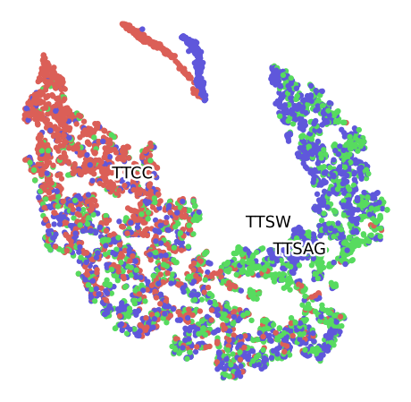
Grouped by Plant
Grouped by Month

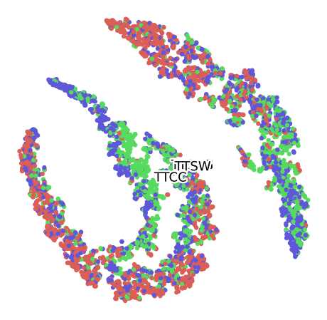
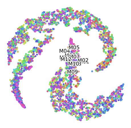
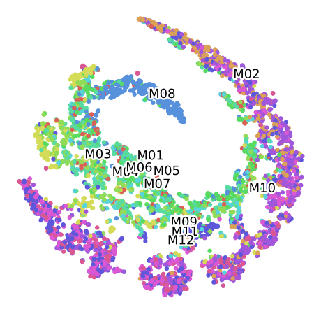
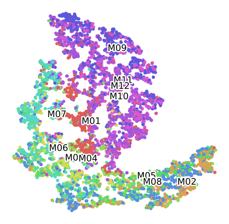
TSNE for the Convolutional Autoencoder (4 Bands)
Grouped by Size
Grouped by Plant
Grouped by Month
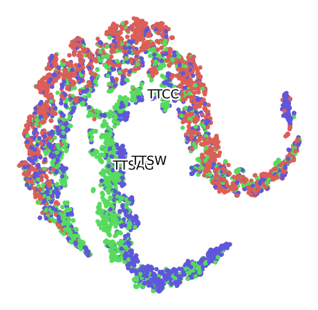
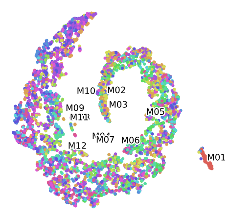
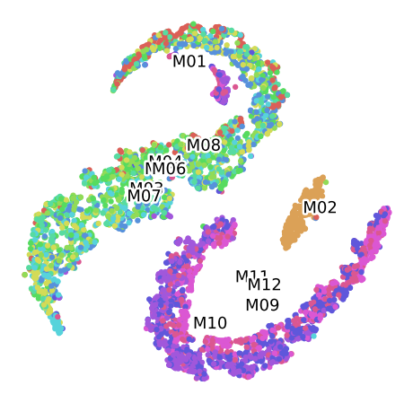
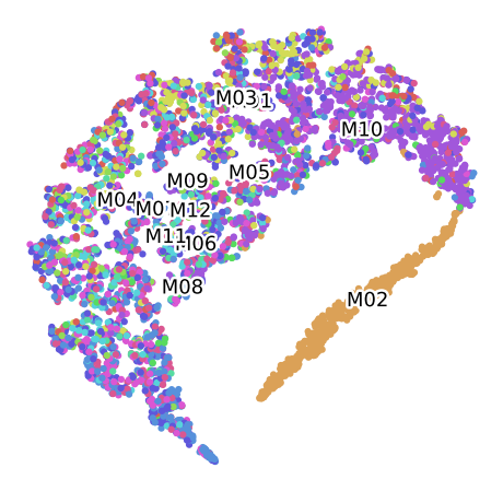
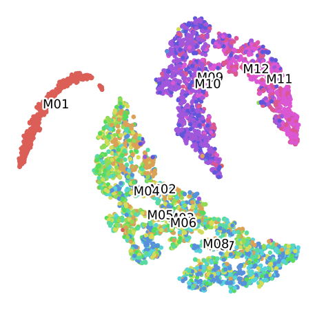
TSNE for the Convolutional Autoencoder (16 Bands)
Grouped by Size
Grouped by Plant
Grouped by Month
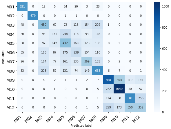
Data splitted by grain size
In order to improve the process, the data will be splitted by the size category. Then samples with granulometry “Minus 100” will be grouped in a set will the other set will to consider the data of granulometry “Plus 100”
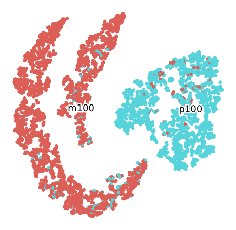
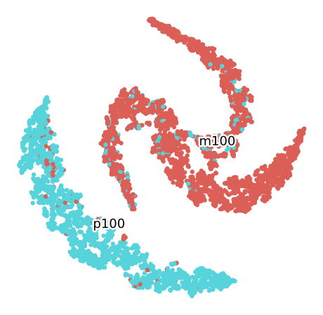
TSNE M100 for the Convolutional Autoencoder (16 Bands)
Clustering of data set M100 Labelled by Plant of origin
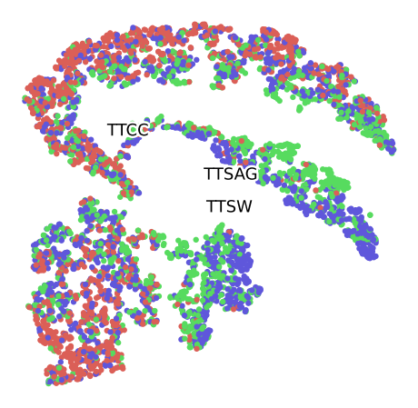
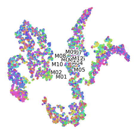
Clustering of data set M100 For the Plant 1, labelled by Month
Clustering of data set M100 For the Plant 2, labelled by Month
Clustering of data set M100 For the Plant 3, labelled by Month
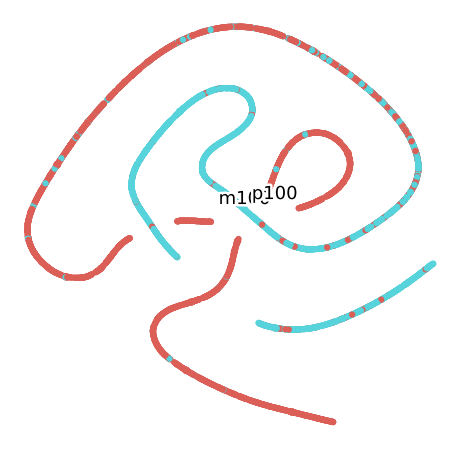
TSNE P100 for the Convolutional Autoencoder (16 Bands)
Clustering of data set P100 Labelled by Plant of origin
Clustering of data set P100 For the Plant 1, labelled by Month
Clustering of data set P100 For the Plant 2, labelled by Month
Clustering of data set P100 For the Plant 3, labelled by Month
Classification of the available categories
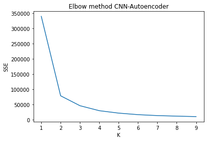
As a reference k-means elbow method was computed to compare the number of clusters for the global data. For all representations the number of clusters estimated was consistent.
from sklearn.cluster import KMeans

def compute_elobow(data, title):
    errors = list()
    for k in tqdm_notebook(range(1, 10)):
        km = KMeans(n_clusters=k, n_jobs=-1)
        km.fit(data)
        errors.append(km.inertia_)
    plot_elbow(errors, title)

def plot_elbow(errors, title):
    fig, ax = plt.subplots()
    ax.plot(np.arange(1, len(errors) + 1), errors)
    ax.set_title(title)
    ax.set_xlabel('K')
    ax.set_ylabel('SSE')
    plt.show()
Performance with PCA reduced data
Classification of Grain Size
         | precision  |  recall | f1-score  | support

       0 |      0.88  |    0.88 |     0.88  |   36198
       1 |      0.84  |    0.84 |     0.84  |   26391

accuracy |            |         |     0.86  |   62589
| macro avg | 0.86 | 0.86 | 0.86 | 62589 |
| weighted avg | 0.86 | 0.86 | 0.86 | 62589 |
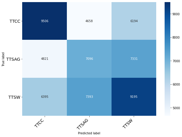
Classification of Origin Plant
         | precision  |  recall | f1-score  | support

       0 |      0.46  |    0.47 |     0.46  |   20358
       1 |      0.37  |    0.37 |     0.37  |   19248
       2 |      0.40  |    0.40 |     0.40  |   22983

accuracy |            |         |     0.41  |   62589
| macro avg | 0.41 | 0.41 | 0.41 | 62589 |
| weighted avg | 0.41 | 0.41 | 0.41 | 62589 |
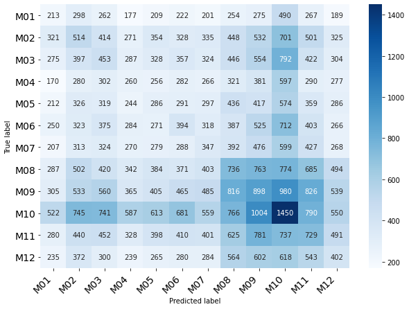
Classification of Month
         | precision  |  recall | f1-score  | support

       0 |      0.06  |    0.07 |     0.07  |    3057
       1 |      0.10  |    0.10 |     0.10  |    5044
       2 |      0.09  |    0.09 |     0.09  |    4939
       3 |      0.07  |    0.07 |     0.07  |    3682
       4 |      0.07  |    0.07 |     0.07  |    4047
       5 |      0.09  |    0.09 |     0.09  |    4508
       6 |      0.08  |    0.08 |     0.08  |    4190
       7 |      0.12  |    0.12 |     0.12  |    6161
       8 |      0.12  |    0.13 |     0.12  |    7177
       9 |      0.16  |    0.16 |     0.16  |    9008
      10 |      0.12  |    0.12 |     0.12  |    6072
      11 |      0.09  |    0.09 |     0.09  |    4704

accuracy |            |         |     0.11  |   62589
| macro avg | 0.10 | 0.10 | 0.10 | 62589 |
| weighted avg | 0.11 | 0.11 | 0.11 | 62589 |
Performance with SAE Autoencoder 4 dims reduced data
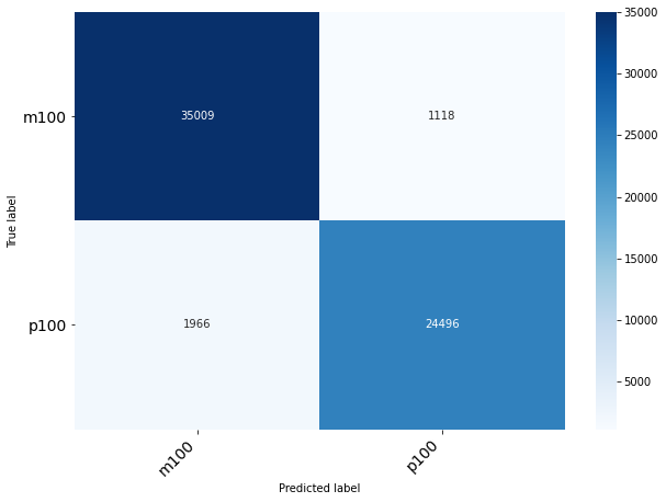
Classification of Grain Size
         | precision  |  recall | f1-score |  support

       0 |      0.95  |    0.97 |     0.96 |    36127
       1 |      0.96  |    0.93 |     0.94 |    26462

accuracy |            |         |     0.95 |    62589
| macro avg | 0.95 | 0.95 | 0.95 | 62589 |
| weighted avg | 0.95 | 0.95 | 0.95 | 62589 |
Classification of Origin Plant
         | precision  |  recall | f1-score |  support

       0 |      0.59  |    0.68 |     0.64 |    20521
       1 |      0.56  |    0.53 |     0.54 |    19083
       2 |      0.55  |    0.50 |     0.53 |    22985

accuracy |            |         |     0.57 |    62589
| macro avg | 0.57 | 0.57 | 0.57 | 62589 |
| weighted avg | 0.57 | 0.57 | 0.57 | 62589 |
Classification of Month
         | precision  |  recall | f1-score  | support

       0 |      0.27  |    0.31 |     0.29  |    3076
       1 |      0.23  |    0.28 |     0.25  |    5088
       2 |      0.22  |    0.25 |     0.23  |    4793
       3 |      0.20  |    0.20 |     0.20  |    3581
       4 |      0.16  |    0.15 |     0.15  |    4108
       5 |      0.21  |    0.19 |     0.20  |    4485
       6 |      0.15  |    0.13 |     0.14  |    4326
       7 |      0.25  |    0.26 |     0.26  |    6202
       8 |      0.25  |    0.24 |     0.24  |    7205
       9 |      0.28  |    0.34 |     0.31  |    8992
      10 |      0.29  |    0.25 |     0.27  |    6111
      11 |      0.18  |    0.13 |     0.15  |    4622

accuracy |            |         |     0.24  |   62589
| macro avg | 0.22 | 0.23 | 0.22 | 62589 |
| weighted avg | 0.23 | 0.24 | 0.23 | 62589 |
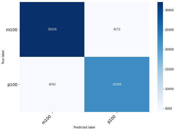
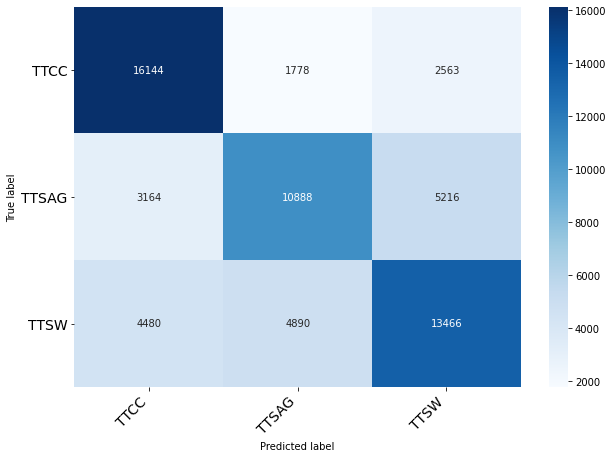
Performance with CNN Autoencoder 16 dims reduced data
Classification of Grain Size
         | precision  |  recall | f1-score |  support

       0 |      0.96  |    0.98 |     0.97 |    36233
       1 |      0.97  |    0.95 |     0.96 |    26356

accuracy |            |         |     0.97 |    62589
| macro avg | 0.97 | 0.97 | 0.97 | 62589 |
| weighted avg | 0.97 | 0.97 | 0.97 | 62589 |

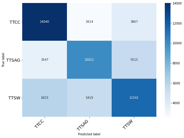
Classification of Origin Plant
         | precision  |  recall | f1-score |  support

       0 |      0.68  |    0.79 |     0.73 |    20485
       1 |      0.62  |    0.57 |     0.59 |    19268
       2 |      0.63  |    0.59 |     0.61 |    22836

accuracy |            |         |     0.65 |    62589
| macro avg | 0.64 | 0.65 | 0.64 | 62589 |
| weighted avg | 0.64 | 0.65 | 0.64 | 62589 |
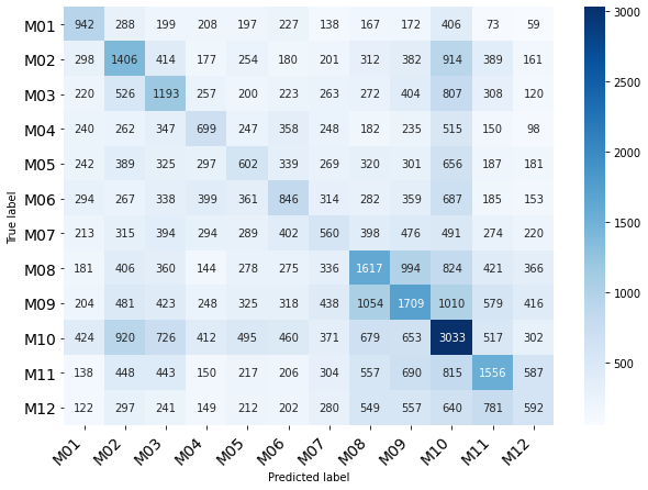
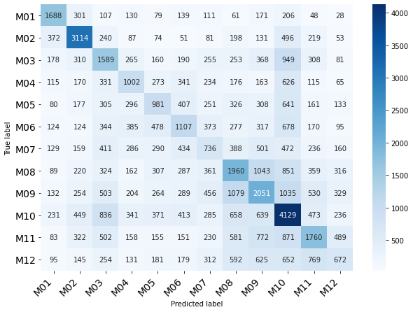
Classification of Month
         | precision  |  recall  | f1-score |  support

       0 |      0.51  |    0.55  |    0.53  |    3069
       1 |      0.54  |    0.61  |    0.57  |    5116
       2 |      0.28  |    0.32  |    0.30  |    4906
       3 |      0.29  |    0.28  |    0.28  |    3611
       4 |      0.27  |    0.24  |    0.26  |    4066
       5 |      0.28  |    0.25  |    0.26  |    4472
       6 |      0.20  |    0.18  |    0.19  |    4202
       7 |      0.30  |    0.31  |    0.31  |    6279
       8 |      0.29  |    0.29  |    0.29  |    7126
       9 |      0.36  |    0.46  |    0.40  |    9061
      10 |      0.34  |    0.29  |    0.31  |    6074
      11 |      0.25  |    0.15  |    0.19  |    4607

accuracy |            |          |    0.33  |   62589
| macro avg | 0.33 | 0.33 | 0.32 | 62589 |
| weighted avg | 0.32 | 0.33 | 0.33 | 62589 |
Final considerations
The final structure has implied a hierarchical system but due to confidentiality issues of the project, the details of the implementation and results are not publicly accessible.
The above results correspond to preliminary tests on the data base.
Some hierarchical clustering modifications can provided information about internal groups in data
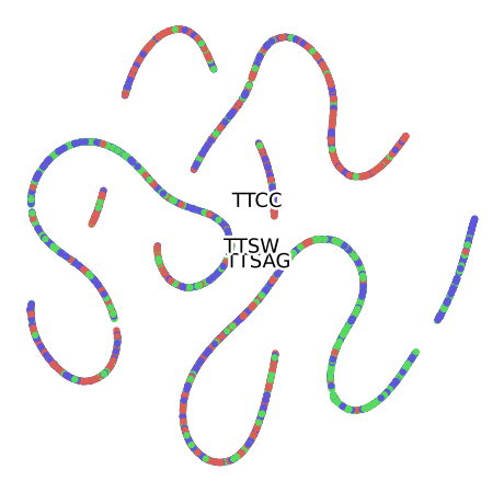
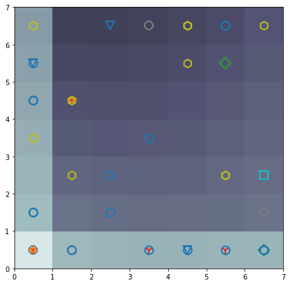
Finally, some experiments were performed using Self Organization Map (SAM) in order to visualizate additional groups in the category related with months
markers = ['o', 's', 'D', '1', '2', '3', '4', '8', 'h', 's', 'v', '*']
colors = ['C0', 'C1', 'C2', 'C3', 'C4', 'C5', 'C6', 'C7', 'C8', 'C9', 'C10', 'C11']
This project was developed as part of the CC5214 Data Science Project course at Universidad de Chile. It does not have a public repository; the data and detailed implementation remain confidential due to the industrial origin of the samples.
Connection to HIDSAG and Geometallurgy
HyClusVi represents an early exploration of the dimensionality reduction and visualization pipeline that later became central to the HIDSAG research program. The insights from this student project – particularly the effectiveness of autoencoder-based spectral compression and t-SNE visualization for mineral discrimination – informed subsequent work on hyperspectral data analysis for geometallurgical estimation. The topic modelling approach presented at Procemin Geomet 2022 builds directly on the spectral representation ideas first tested here, extending them with probabilistic models (LDA) for mineral abundance estimation from SWIR and VNIR imagery.